install.packages("sparseR")
library(sparseR)But what about interactions; are any of those significant?
I have heard some variant of this question from clinicians and researchers from many fields of science. While usually asked in earnest, this question is a dangerous one; the sheer number of interactions can greatly inflate the number of false discoveries in the interactions, resulting in difficult-to-interpret models with many unnecessary interactions. Still, there are times when these expeditions are necessary and fruitful. Thankfully, useful tools are now available to help with the process. This article discusses two regularization-based approaches: Group-Lasso INTERaction-NET (glinternet) and the Sparsity-Ranked Lasso (SRL). The glinternet method implements a hierarchy-preserving selection and estimation procedure, while the SRL is a hierarchy-preferring regularization method which operates under ranked sparsity principles (in short, ranked sparsity methods ensure interactions are treated more skeptically than main effects a priori).
Useful package #1: ranked sparsity methods via sparseR
The sparseR package has been designed to make dealing with interactions and polynomials much more analyst-friendly. Building on the recipes package, sparseR has many built-in tools to facilitate the prepping of a model matrix with interactions and polynomials; these features are presented in the package website located at https://petersonr.github.io/sparseR/. The package is available on CRAN and can be installed and loaded with the code below
The simplest way to implement the SRL in sparseR is via a single call to the sparseR() function, here demonstrated with Fisher’s iris data set. 10-fold cross-validation is used by default, so we set the seed = 1 here for reproducibility.
data(iris)
srl <- sparseR(Sepal.Width ~ ., data = iris, k = 1, seed = 1)
srl
Model summary @ min CV:
-----------------------------------------------------
  lasso-penalized linear regression with n=150, p=21
  (At lambda=0.0024):
    Nonzero coefficients: 7
    Cross-validation error (deviance): 0.07
    R-squared: 0.63
    Signal-to-noise ratio: 1.71
    Scale estimate (sigma): 0.264

  SR information:
             Vartype Total Selected Saturation Penalty
         Main effect     6        2      0.333    2.45
 Order 1 interaction    12        3      0.250    3.46
  Order 2 polynomial     3        2      0.667    3.00


Model summary @ CV1se:
-----------------------------------------------------
  lasso-penalized linear regression with n=150, p=21
  (At lambda=0.0070):
    Nonzero coefficients: 6
    Cross-validation error (deviance): 0.08
    R-squared: 0.58
    Signal-to-noise ratio: 1.39
    Scale estimate (sigma): 0.281

  SR information:
             Vartype Total Selected Saturation Penalty
         Main effect     6        2      0.333    2.45
 Order 1 interaction    12        2      0.167    3.46
  Order 2 polynomial     3        2      0.667    3.00
The summary function produces additional details:
summary(srl, at = "cv1se")lasso-penalized linear regression with n=150, p=21
At lambda=0.0070:
-------------------------------------------------
Nonzero coefficients : 6
Expected nonzero coefficients: 0.44
Average mfdr (6 features) : 0.074
Estimate z mfdr Selected
Species_setosa 0.82889 18.596 < 1e-04 *
Sepal.Length_poly_1 0.19494 9.638 < 1e-04 *
Petal.Width_poly_2 0.10142 4.698 0.00016138 *
Petal.Width:Species_versicolor 0.29190 3.335 0.02568952 *
Sepal.Length:Species_setosa 0.06826 2.769 0.14613161 *
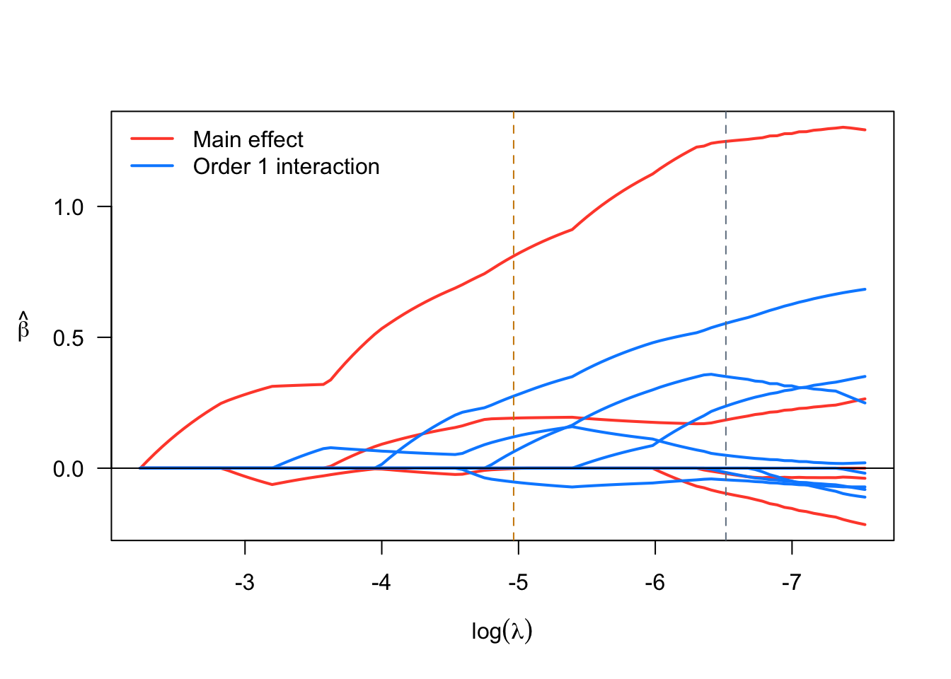
Sepal.Length_poly_2 -0.03215 -2.694 0.27005358 *We see that two models are displayed by default corresponding to two “smart” choices for the penalization parameter \(\lambda\). The first model printed refers to the model where \(\lambda\) is set to minimize the cross-validated error, while the second one refers to a model where \(\lambda\) is set to a value such that the model is as sparse as possible while still being within 1 SD of the minimum cross-validated error. Visualizations are also available via sparseR that can help visualize both the solution path and the resulting model (interactions can be very challenging to interpret without a good figure!)
plot(srl)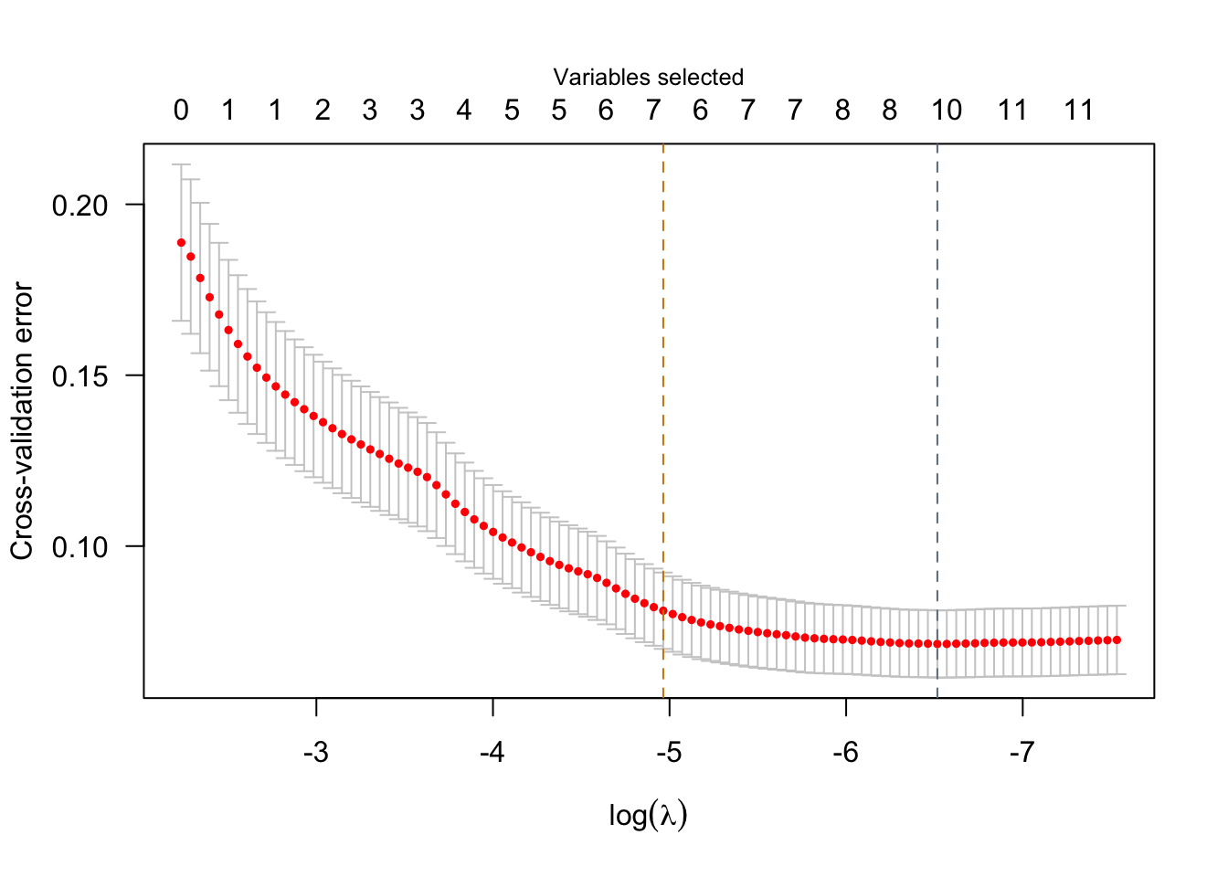
effect_plot(srl, "Petal.Width", by = "Species", at = "cvmin")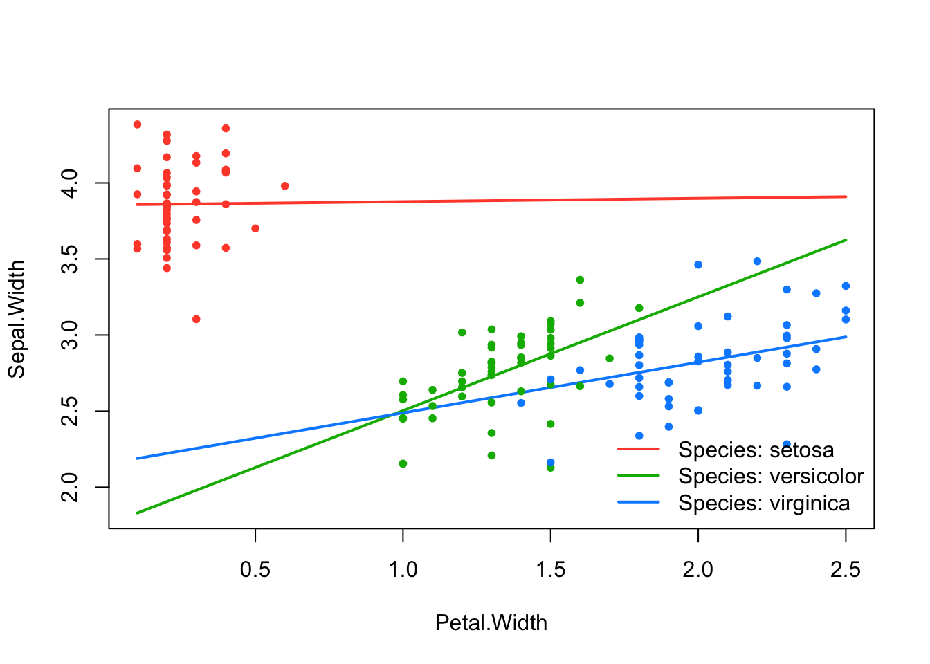
effect_plot(srl, "Petal.Width", by = "Species", at = "cv1se")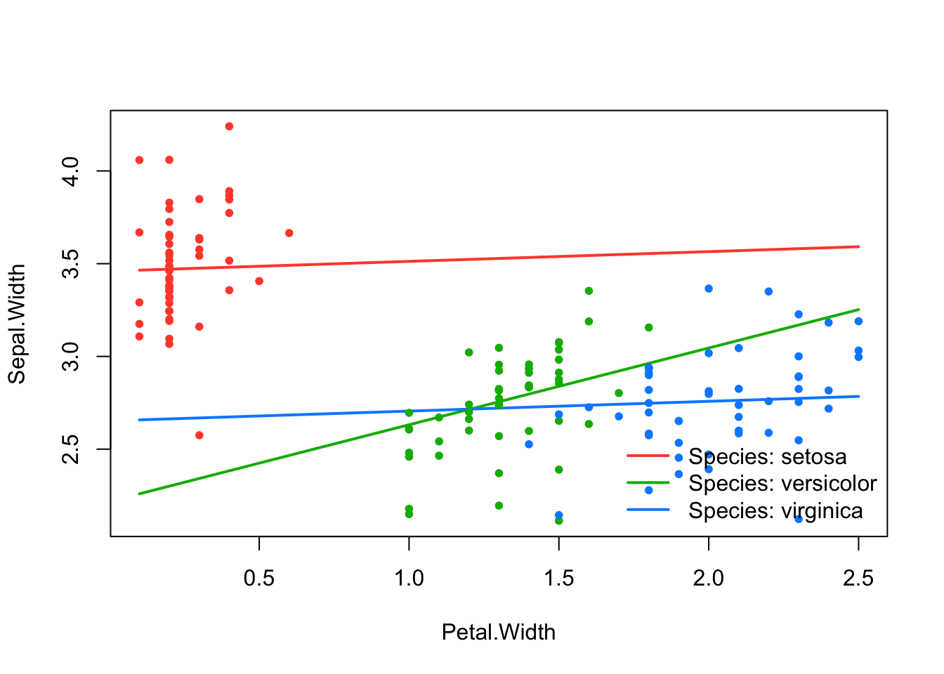
Note that while ranked sparsity principles were motivated by the estimation of the lasso (Peterson & Cavanaugh 2022), they can also be implemented with MCP, SCAD, or elastic net and for binary, normal, and survival data. Finally, sparseR includes some functionality to perform forward-stepwise selection using a sparsity-ranked modification of BIC, as well as post-selection inferential techniques using sample splitting and bootstrapping.
Useful package #2: hierarchy-preserving regularization via glinternet
Some argue that when it comes to interactions, hierarchy is very important (i.e., an interaction shouldn’t be included in a model without its constituent main effects). While ranked sparsity methods do prefer hierarchical models, they can often still produce non-hierarchical ones. The glinternet package and the function of the same name uses regularization for model selection under hierarchy constraint, such that all candidate models are hierarchical. Glinternet can handle both continuous and categorical predictors, but requires pre-specification of a numeric model matrix. It can be performed as follows:
# install.packages("glinternet")
library(glinternet)
library(dplyr)

X <- iris %>%
  select(-Sepal.Width) %>%
  mutate(Species = as.numeric(Species) - 1)

set.seed(321)
cv_fit <- glinternet.cv(X, Y = iris$Sepal.Width, numLevels = c(1,1,1,3))
The cv_fit object contains necessary information from the cross-validation procedure and the fits themselves stored in a series of lists. A more in-depth tutorial to extract coefficients (and facilitate a model interpretation) using the glinternet package can be found at https://strakaps.github.io/post/glinternet/. Importantly, both the glinternet and sparseR methods have associated predict methods which can yield predictions on new (or the training) data, shown below. For comparison, we also fit a “main effects only” model with sparseR by setting k = 0.
me <- sparseR(Sepal.Width ~ ., data = iris, k = 0, seed = 333)
p_me <- predict(me)
p_srl <- predict(srl)
p_gln <- as.vector(predict(cv_fit, X))
With a little help from the yardstick package’s metrics() function, we can compare the accuracy of each model’s predictions using root-mean-squared error (RMSE), R-squared (RSQ), and mean absolute error (MAE); see table below. Evidently, glinternet and SRL are similar in terms of their predictive performance. However, both outperform the main effects model considerably, suggesting interactions among other variables do have signal worth capturing when predicting Sepal.Width.
gln_res <- tibble(p_gln, y = iris$Sepal.Width) %>%
  yardstick::metrics(y, p_gln) %>%
  rename("glinternet"= .estimate)
srl_res <- tibble(p_srl, y = iris$Sepal.Width) %>%
  yardstick::metrics(y, p_srl) %>%
  rename("SRL"= .estimate)
me_res <- tibble(p_me, y = iris$Sepal.Width) %>%
  yardstick::metrics(y, p_me) %>%
  rename("Main effects only"= .estimate)

results_table <- gln_res %>%
  bind_cols(srl_res[,3]) %>%
  bind_cols(me_res[,3]) %>%
  rename("Metric" = .metric) %>%
  mutate(Metric = toupper(Metric)) %>%
select(-.estimator)| Metric | glinternet | SRL | Main effects only |
|---|---|---|---|
| RMSE | 0.24 | 0.25 | 0.25 |
| RSQ | 0.69 | 0.68 | 0.66 |
| MAE | 0.19 | 0.19 | 0.19 |
Other packages worth mentioning: ncvreg, hierNet, visreg, sjPlot
The SRL and other sparsity-ranked regularization methods implemented in sparseR would not be possible without the ncvreg package, which performs the heavy-lifting in terms of model fitting, optimization, and cross-validation. The hierNet package is another hierarchy-enforcing procedure that may yield better models than glinternet, however the latter is more computationally efficient especially for situations with a medium-to-large number of covariates. Finally, when interactions or polynomials are included in models, figures are truly worth a thousand words, and packages such as visreg and sjPlot have great functionality for plotting the effects of interactions.
References
- Bien J and Tibshirani R (2020). hierNet: A Lasso for Hierarchical Interactions. R package version 1.9. https://CRAN.R-project.org/package=hierNet
- Breheny P and Burchett W (2017). Visualization of Regression Models Using visreg. The R Journal, 9: 56-71.
- Breheny P and Huang J (2011). Coordinate descent algorithms for nonconvex penalized regression, with applications to biological feature selection. Ann. Appl. Statist., 5: 232-253.
- Kuhn M and Vaughan D (2021). yardstick: Tidy Characterizations of Model Performance. R package version 0.0.8. https://CRAN.R-project.org/package=yardstick
- Lim M and Hastie T (2020). glinternet: Learning Interactions via Hierarchical Group-Lasso Regularization. R package version 1.0.11. https://CRAN.R-project.org/package=glinternet
- Lüdecke D (2021). sjPlot: Data Visualization for Statistics in Social Science. R package version 2.8.8. https://CRAN.R-project.org/package=sjPlot
- Peterson R (2021). sparseR: Variable selection under ranked sparsity principles for interactions and polynomials. https://github.com/petersonR/sparseR/.
- Peterson, R, Cavanaugh, J. Ranked sparsity: a cogent regularization framework for selecting and estimating feature interactions and polynomials. AStA Adv Stat Anal 106, 427–454 (2022). https://doi.org/10.1007/s10182-021-00431-7
Note
This post was originally published in the Biometric Bulletin (2021) Volume 38 Issue 3.
Appendix
R Session Info
sessioninfo::session_info()─ Session info ───────────────────────────────────────────────────────────────
setting value
version R version 4.5.2 (2025-10-31)
os macOS Tahoe 26.4.1
system aarch64, darwin20
ui X11
language (EN)
collate en_US.UTF-8
ctype en_US.UTF-8
tz America/Chicago
date 2026-04-28
pandoc 3.6.3 @ /Applications/RStudio.app/Contents/Resources/app/quarto/bin/tools/aarch64/ (via rmarkdown)
quarto 1.8.25 @ /Applications/RStudio.app/Contents/Resources/app/quarto/bin/quarto
─ Packages ───────────────────────────────────────────────────────────────────
package * version date (UTC) lib source
class 7.3-23 2025-01-01 [2] CRAN (R 4.5.2)
cli 3.6.5 2025-04-23 [1] CRAN (R 4.5.0)
codetools 0.2-20 2024-03-31 [2] CRAN (R 4.5.2)
data.table 1.18.2.1 2026-01-27 [1] CRAN (R 4.5.2)
digest 0.6.39 2025-11-19 [1] CRAN (R 4.5.2)
dplyr * 1.2.0 2026-02-03 [1] CRAN (R 4.5.2)
evaluate 1.0.5 2025-08-27 [1] CRAN (R 4.5.0)
farver 2.1.2 2024-05-13 [1] CRAN (R 4.5.0)
fastmap 1.2.0 2024-05-15 [1] CRAN (R 4.5.0)
future 1.70.0 2026-03-14 [1] CRAN (R 4.5.2)
future.apply 1.20.2 2026-02-20 [1] CRAN (R 4.5.2)
generics 0.1.4 2025-05-09 [1] CRAN (R 4.5.0)
glinternet * 1.0.12 2021-09-03 [1] CRAN (R 4.5.0)
globals 0.19.1 2026-03-13 [1] CRAN (R 4.5.2)
glue 1.8.0 2024-09-30 [1] CRAN (R 4.5.0)
gower 1.0.2 2024-12-17 [1] CRAN (R 4.5.0)
hardhat 1.4.2 2025-08-20 [1] CRAN (R 4.5.0)
htmltools 0.5.9 2025-12-04 [1] CRAN (R 4.5.2)
htmlwidgets 1.6.4 2023-12-06 [1] CRAN (R 4.5.0)
ipred 0.9-15 2024-07-18 [1] CRAN (R 4.5.0)
jsonlite 2.0.0 2025-03-27 [1] CRAN (R 4.5.0)
kableExtra * 1.4.0 2024-01-24 [1] CRAN (R 4.5.0)
knitr 1.50 2025-03-16 [1] CRAN (R 4.5.0)
lattice 0.22-7 2025-04-02 [2] CRAN (R 4.5.2)
lava 1.8.2 2025-10-30 [1] CRAN (R 4.5.0)
lifecycle 1.0.5 2026-01-08 [1] CRAN (R 4.5.2)
listenv 0.10.1 2026-03-10 [1] CRAN (R 4.5.2)
lubridate 1.9.5 2026-02-04 [1] CRAN (R 4.5.2)
magrittr 2.0.5 2026-04-04 [1] CRAN (R 4.5.2)
MASS 7.3-65 2025-02-28 [2] CRAN (R 4.5.2)
Matrix 1.7-4 2025-08-28 [2] CRAN (R 4.5.2)
ncvreg 3.16.0 2025-10-09 [1] Github (pbreheny/ncvreg@5fecc8c)
nnet 7.3-20 2025-01-01 [1] CRAN (R 4.5.0)
parallelly 1.46.1 2026-01-08 [1] CRAN (R 4.5.2)
pillar 1.11.1 2025-09-17 [1] CRAN (R 4.5.0)
pkgconfig 2.0.3 2019-09-22 [1] CRAN (R 4.5.0)
prodlim 2026.03.11 2026-03-11 [1] CRAN (R 4.5.2)
purrr 1.2.1 2026-01-09 [1] CRAN (R 4.5.2)
R6 2.6.1 2025-02-15 [1] CRAN (R 4.5.0)
RColorBrewer 1.1-3 2022-04-03 [1] CRAN (R 4.5.0)
Rcpp 1.1.1 2026-01-10 [1] CRAN (R 4.5.2)
recipes 1.3.1 2025-05-21 [1] CRAN (R 4.5.0)
rlang 1.1.7 2026-01-09 [1] CRAN (R 4.5.2)
rmarkdown 2.30 2025-09-28 [1] CRAN (R 4.5.0)
rpart 4.1.24 2025-01-07 [2] CRAN (R 4.5.2)
rstudioapi 0.17.1 2024-10-22 [1] CRAN (R 4.5.0)
scales 1.4.0 2025-04-24 [1] CRAN (R 4.5.0)
sessioninfo 1.2.3 2025-02-05 [1] CRAN (R 4.5.0)
sparseR * 0.3.2 2025-04-14 [1] CRAN (R 4.5.0)
sparsevctrs 0.3.6 2026-01-27 [1] CRAN (R 4.5.2)
stringi 1.8.7 2025-03-27 [1] CRAN (R 4.5.0)
stringr 1.6.0 2025-11-04 [1] CRAN (R 4.5.0)
survival 3.8-3 2024-12-17 [2] CRAN (R 4.5.2)
svglite 2.2.2 2025-10-21 [1] CRAN (R 4.5.0)
systemfonts 1.3.1 2025-10-01 [1] CRAN (R 4.5.0)
textshaping 1.0.4 2025-10-10 [1] CRAN (R 4.5.0)
tibble 3.3.1 2026-01-11 [1] CRAN (R 4.5.2)
tidyr 1.3.2 2025-12-19 [1] CRAN (R 4.5.2)
tidyselect 1.2.1 2024-03-11 [1] CRAN (R 4.5.0)
timechange 0.4.0 2026-01-29 [1] CRAN (R 4.5.2)
timeDate 4052.112 2026-01-28 [1] CRAN (R 4.5.2)
vctrs 0.7.2 2026-03-21 [1] CRAN (R 4.5.2)
viridisLite 0.4.3 2026-02-04 [1] CRAN (R 4.5.2)
withr 3.0.2 2024-10-28 [1] CRAN (R 4.5.0)
xfun 0.54 2025-10-30 [1] CRAN (R 4.5.0)
xml2 1.5.1 2025-12-01 [1] CRAN (R 4.5.2)
yaml 2.3.11.9000 2025-12-10 [1] Github (r-lib/r-yaml@6dc4582)
yardstick 1.3.2 2025-01-22 [1] CRAN (R 4.5.0)
[1] /Users/rpterson/Library/R/arm64/4.5/library
[2] /Library/Frameworks/R.framework/Versions/4.5-arm64/Resources/library
* ── Packages attached to the search path.
──────────────────────────────────────────────────────────────────────────────Citation
For attribution, please cite this work as:
Peterson, Ryan. 2023. “Detecting Interactions in R.”
Data Diction (blog). June 20, 2023. https://doi.org/10.59350/f11j1-neh89.
